Advanced Deep Learning for computer vision

Focus will be on Image Segmentation

Be warned…. training this deep learning model will take much longer than all of the other ones we’ve done so far.

So far, we’ve focused on image classification models: basically, an image goes in, a label comes out. But, image classification is only one of several possible applications of deep learning in computer vision. In general, there are 3 essential computer vision tasks you need to know about:

• Image Classification - Where the goal is to assign 1 or more labels to an image. It may be either single-label classification, or multi-label classification.

• Image Segmentation - Where the goal is to “segment” or “partition” an image into different areas, with each area usually representing a category.

• Object Detection - Where the goal is to draw rectangles (called bounding boxes) around objects of interest in an image, and associate each rectangle with a class. A self-driving car could use an object-detection model to monitor cars, pedestrians, and signs in view of its cameras.

A diagram of the difference between the 3 is below.

For this post, we’ll focus on Image Segmentation

2 Flavors of image segmentation

Image segmentation with deep learning is about using a model to assign a class to each pixel in an image, thus “segmenting” the image into different zones (ie “background” and “foreground”, or “road”, “car”, and “sidewalk)

There are 2 flavors of image segmentation that you should know about:

• Semantic Segmentation: Where each pixel is independently classified into a semantic category, like “cat”. If there are 2 cats in the image, the corresponding pixels are all mapped to the same generic “cat” category.

• Instance Segmentation: It seeks not only to classify image pixels by category, but also to parse out individual object instances. In an image with 2 cats in it, instance segmentation would treat “cat 1”, and “cat 2” as 2 separate classes of pixels.

For this specific post, we’ll be focusing on semantic segmentation. We’ll be looking at images of cats, and dogs, and this time we’ll learn how to tell apart the main subject and it’s background.

Fetching the data

We’ll be using the Oxford-3T pets dataset: https://www.robots.ox.ac.uk/~vgg/data/pets/

You can download the images here: http://www.robots.ox.ac.uk/~vgg/data/pets/data/images.tar.gz

You can download the annotations here:
http://www.robots.ox.ac.uk/~vgg/data/pets/data/annotations.tar.gz

Once you have done that, you’ll want to go ahead and extract those zip files. You’ll now have 2 folders called “images”, and “annotations”

Great, let’s get started and load up our data. We’ll be focusing on first getting a list of input file paths, as well as their respective list of the mask file paths.

Data exploration

Here’s the python code we are using to prep our list of data

import os
input_dir = 'images/'
target_dir = 'annotations/trimaps/'

input_img_paths = sorted(
    [os.path.join(input_dir, fname)
     for fname in os.listdir(input_dir)
     if fname.endswith('.jpg')])

target_paths = sorted(
    [os.path.join(target_dir, fname)
     for fname in os.listdir(target_dir)
     if fname.endswith('.png') and not fname.startswith('.')])

Now, let’s take a look at what one of these inputs, and it’s mask looks like. Let’s load up one of our images:

import matplotlib.pyplot as plt
from tensorflow.keras.utils import load_img, img_to_array
from PIL import Image

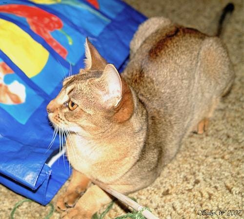
img = load_img(input_img_paths[9])
img_array = img_to_array(img)
img_pil = Image.fromarray(img_array.astype('uint8'))
img_pil.save('asdf.jpg')

here’s what image number 9 looks like:

Now, let’s take a look at the masking layer:

def save_target(target_array, save_path='asdf.jpg'):
    normalized_array = (target_array.astype('uint8') - 1) * 127
    img_to_save = Image.fromarray(normalized_array[:, :, 0], mode='L')
    img_to_save.save(save_path)

img = img_to_array(load_img(target_paths[9], color_mode='grayscale'))
save_target(img)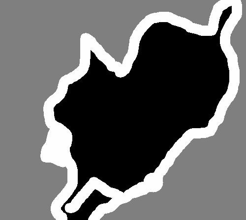

Voila, welcome to image segmentation, now let’s prepare the data

Data prep

For this, we’ll be resizing everything to 200x200.

import numpy as np
import random

img_size = (200, 200)
num_imgs = len(input_img_paths)
random.Random(1337).shuffle(input_img_paths)
random.Random(1337).shuffle(target_paths)

Then, we’ll be loading all images and their masks.

def path_to_input_image(path):
    return img_to_array(load_img(path, target_size = img_size))

def path_to_target(path):
    img = img_to_array(
        load_img(path, target_size= img_size, color_mode = 'grayscale'))
    img = img.astype('uint8') - 1
    return img

input_imgs = np.zeros((num_imgs, ) + img_size + (3, ), dtype='float32')
targets = np.zeros((num_imgs, ) + img_size + (1,), dtype = 'uint8')

for i in range(num_imgs):
    input_imgs[i] = path_to_input_image(input_img_paths[i])
    targets[i] = path_to_target(target_paths[i])

Now, we’ll do the train, test split.

num_val_samples = 1000
train_input_imgs = input_imgs[:-num_val_samples]
train_targets = targets[: -num_val_samples]
val_input_imgs = input_imgs[-num_val_samples:]
val_targets = targets[-num_val_samples:]

Model definition

Now that the data is ready to rock, let’s start working on our model definition. One thing to keep in mind is that each pixel in our output will actually have 3 layers, if you think about it, it makes sense. We are trying to basically predict 3 layers in the entire image:

1. Background - Grey color

2. Border - White Border

3. Our Object - In Black

you can scroll up to see our cat’s mask to visualize the 3 layers. Now… let’s get to work on constructing the model

from tensorflow import keras
from tensorflow.keras import layers

def get_model(img_size, num_classes):
    inputs = keras.Input(shape = img_size + (3,))
    x = layers.Rescaling(1./255)(inputs)

    x = layers.Conv2D(64, 3, strides = 2, activation = 'relu', padding = 'same')(x)
    x = layers.Conv2D(64, 3, activation = 'relu', padding = 'same')(x)
    x = layers.Conv2D(128, 3, strides = 2, activation = 'relu', padding = 'same')(x)
    x = layers.Conv2D(128, 3, activation = 'relu', padding = 'same')(x)
    x = layers.Conv2D(256, 3, strides = 2, activation = 'relu', padding = 'same')(x)
    x = layers.Conv2D(256, 3, activation = 'relu', padding = 'same')(x)

    x = layers.Conv2DTranspose(256, 3, activation = 'relu', padding = 'same')(x)
    x = layers.Conv2DTranspose(256, 3, activation = 'relu', padding = 'same', strides = 2)(x)
    x = layers.Conv2DTranspose(128, 3, activation = 'relu', padding = 'same')(x)
    x = layers.Conv2DTranspose(128, 3, activation = 'relu', padding = 'same', strides = 2)(x)
    x = layers.Conv2DTranspose(64, 3, activation = 'relu', padding = 'same')(x)
    x = layers.Conv2DTranspose(64, 3, activation = 'relu', padding = 'same', strides = 2)(x)

    outputs = layers.Conv2D(num_classes, 3, activation = 'softmax', padding = 'same')(x)
    model = keras.Model(inputs, outputs)
    return model

model = get_model(img_size = img_size, num_classes= 3)

And, here’s a preview of the model summary

If you’ve been keeping up with the other deep learning posts, then this is nothing special, the biggest change is that in the image classification tasks, we used a MaxPooling2D layer to downsample feature maps. Here, we downsample by adding strides to every other convolution layer.

The reason we do this is because, in the case of image segmentation, we care a lot about the spatial location of information in the image, since we need to produce per-pixel target masks as output of the model. When you do a 2x2 max pooling, you completely destroy all location information within each pooling window.

Once we have downsampled our data, we’ll want to upsample the analysis to get it back into the 200x200 pixel shape. To do this, we use the Conv2DTranspose layers. It’s effectively an inverse of a dowsample, visualized below:

Model fit & prediction

We can now compile and fit our model, we’ll use a simple callback as well to save only the best performing model (based on epoch):

model.compile(optimizer='rmsprop', loss = 'sparse_categorical_crossentropy')
callbacks = [keras.callbacks.ModelCheckpoint('oxfort_segmentation.keras', save_best_only=True)]
history = model.fit(train_input_imgs, train_targets,
                    epochs=50,
                    callbacks=callbacks,
                    batch_size = 64,
                    validation_data = (val_input_imgs, val_targets))

And, here’s how you can get it to predict on some data:

from tensorflow.keras.utils import array_to_img
from PIL import Image
import numpy as np

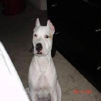
i = 4
test_image = val_input_imgs[i]
input_img_pil = array_to_img(test_image)
input_img_pil.save('input_image.jpg')

mask = model.predict(np.expand_dims(test_image, 0))[0]

def save_mask(pred, save_path='predicted_mask.jpg'):
    mask = np.argmax(pred, axis=-1)
    mask_img = (mask * 127).astype(np.uint8)
    mask_pil = Image.fromarray(mask_img)
    mask_pil.save(save_path)

save_mask(mask)

Here is the image, and the mask side by side of our prediction.

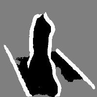
computer did a restart overnight (thanks windows), but you can see if the epochs kept continuing the mask would converge to the appropriate photo.