Anova Regression

Anova Regression: What is it? How do you implement it, what are t-tests, and everything else you need to know.

You can view the code used for this post here

The most important thing with Anova is not the regression equation behind it, but rather being able to actually implement it in code, and read what information the table is telling you.

Remember, we all use computers nowadays, so realistically speaking no one will ever have to calculate any of this by hand (unless you are in University), we just program it in, and have them take care of it. This post focuses heavily onto the theory as some people like to know the mathematics behind the technique to see what’s going on in there.

If you are going for a research heavy job, they’ll probably probe you a little bit on the theory here, if you are going for more of a profit focused role, all they care about is the implementation.

Note: For this whole post, when we refer to linear regression, we are just keeping things super simple and just talking about the normal multiple linear regression, we are not talking about the stepwise regression.

Table of Contents:

1. Frequently Asked Questions

2. Implementation of ANOVA model & Feature Selection using P-Value

3. ANOVA Regression

4. ANOVA model (More Theory)

5. Square Error

1. Frequently Asked Questions:

1. What is the difference between regression and ANOVA?

   1. ANOVA (Analysis of Variance) is a technique used to compare the means of two or more groups. The assumption behind ANOVA is that the groups are sampled from populations that have the same distribution. If this assumption is violated, then the results of the ANOVA should be interpreted with caution.

      Regression is a technique used to model relationships between two or more variables. The regression line will slope in the direction of the strongest relationship and will have an intercept that represents the mean value of y when x is equal to 0. If you need a bit of a review on how linear regression actually works (the mathematics behind it) click here.

2. How do you do an ANOVA table in multiple regression?

   1. To produce an ANOVA table in multiple regression, you first need to calculate the variance inflation factor (VIF) for each independent variable. The VIF measures how much each independent variable inflates the variance of the dependent variable. You then enter these values into a table, together with the R-squared value and the F-statistic.

3. How is ANOVA a linear model?

   1. Anova is a linear model because it looks at the relationship between two variables and how they vary together. In particular, Anova can be used to determine whether there is a significant difference between the means of two groups.

      An example of this would be if you were interested in determining whether there was a significant difference between the heights of men and women. You could use Anova to see if there was a statistically significant difference between the average height of men and women.

      Generally speaking, Anova tests are Linear Models because they involve some kind of dependent variable that can be predicted from an independent variable (in our case, the gender identifiers)

4. What does ANOVA table tell us in multiple regression?

   1. The ANOVA table in multiple regression tells us how much of the variation in the outcome variable (Y) is accounted for by the predictor variables (X1, X2, … , Xk).

      The ANOVA table also tells us whether any of the predictor variables are statistically significant. If a predictor variable is not statistically significant, it can be safely eliminated from the model. In other words, ANOVA is great for figuring out which predictor (x-columns) to keep, and which ones to discard.

5. Should I use ANOVA or regression?

   1. The answer to this question depends on the type of data you are working with and your objectives. If you are working with continuous data and your objective is to predict a continuous outcome variable, then regression is the appropriate technique. If you are working with categorical data and your objective is to compare means across groups, then ANOVA is the appropriate technique.

2. Implementation of ANOVA model & Feature Selection Using P-Value

We'll be using R which is a solid statistical software, and is amazing for anova, and Python, which although not as amazing can still give us the results.

R

Loading our data

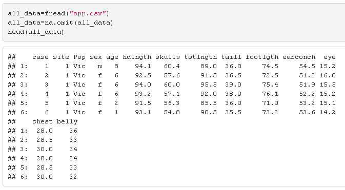
We'll load up the oppossum data that we've been working with for quite a while now.

You can get the data by clicking here.

Setting up the regression variables & Categorical variables

The first thing we would like to do is run a simple regression line, and then see which of all of these variables from stepwise regression are actually making a significant enough of an impact to hold onto.

To keep things simple, we'll run this giant paragraph for data tweaking. It may look long and complicated, but all it's really doing is just tweaking our data up a bit, and using feature engineering to squeeze out as much value as possible from our data.

Running a Linear regression model

Let's run a linear model by doing lm(). FYI, this is the same model from the last stepwise regression.

Examining the Regression statistics

From the above let's take a look at some of the conclusions we can gather right away:

• The p-value for the numerical columns is around 0.1, and for categorical columns it's huge. This means that the newly added explanatory variables (categorical) that we added in were so bad.... they started taking away from the numerical values. So, creating a bunch of dummy variables here is not going to cut it.

• F-Statistic: If you wanted to know what the F-static is for your dataset, this is available here.

• The Multiple R-Squared and Adjusted R-Squared is a simple measure of the goodness of fit. Long story short, even this metric is telling us this model is awful.

TLDR: Basically although we ran a lot of feature engineering, it seemed like it was doing great, from the above metrics we can see it was pretty bad, and a lot of newly created explanatory variable take the blame.

So, let's go on ahead, and run a simple ANOVA model on our explanatory variable (categorical), and see if it is even worth holding onto the categorical data.

Running 1 Way ANOVA

In order to run a 1 way analysis of variance on our explanatory variable, we will use the aov() function. Simply point out the predictor and explanatory variable, and the dataset.

Now with the model run, let's examine the details we can gather from it. We can use the summary() function on the model.

From the above, we can quickly examine and see that the p-value of sex is greater than 0.05. In other words, this tells us that the explanatory variable (sex) is useless for predicting the age. And if you think about it, it kind of makes sense. If I told you I was a male, could you predict my age with just that info?

Running 2 Way Anova

Now, let's run a simple 2 way Analysis of variance linear model. We'll first make our case column to be a string, now let's take a look. Code for this is essentially the same.

Now, let's take a look at the conclusion this provides us by using the summary() function on our model.

Now that we've loaded up our 2 way analysis of variance, now let's take a look at the numeric values in the table and see what they mean.

We will use the summary() function on the model above.

The above tells us that using either sex, or using the Pop column is still pretty useless for trying to figure out the age of an opposum. In conclusion, we have now run two different tests that basically showed us the using the dummy variables approach for this dataset was a dead end basically.

Python

Loading our data

Let's load up the libraries needed to run the regression line, and the anova model.

You can get the data by clicking here.

Setting up the regression variables & Categorical variables

Now, we'll set these up in a similar way that we did in the previous stepwise regression model.

Running a Linear regression model

Here, we'll do something a little different, last time we used the sklearn library to run the regression model. This time, we'll actually use the statsmodels library instead. This is because this library has several features we are looking for including the test statistic.

Now, let's split the data into the X and Y sets, and use the library to run the regression analysis.

Examining the Regression Coefficients

Now let's examine what the regression coefficients are telling us real quick.

From the above let's take a look at some of the conclusions we can gather right away:

• The p-value for the numerical columns is around 0.1, and for categorical columns it's huge. This means that the newly added explanatory variables (categorical) that we added in were so bad.... they started taking away from the numerical values. So, creating a bunch of dummy variables here is not going to cut it.

• F-Statistic: If you wanted to know what the F-static is for your dataset, this is available here.

• The Multiple R-Squared and Adjusted R-Squared is a simple measure of the goodness of fit. Long story short, even this metric is telling us this model is awful.

TLDR: Basically although we ran a lot of feature engineering, it seemed like it was doing great, from the above metrics we can see it was pretty bad, and a lot of newly created explanatory variable take the blame.

So, let's go on ahead, and run a simple ANOVA model on our explanatory variable (categorical), and see if it is even worth holding onto the categorical data.

Running 1 way anova

We'll use the ols() function from the statsmodel library to do this.

Now, let's take a look at the results from the above

The TLDR of this is that using just sex on it's own is not a good metric to see if we can predict the age.

Running 2 way anova

The code for running the 2 way approach is roughly the same, just add in the extra dummy variables. Here is the code below.

Now, let's look at the results.

The above tells us that using either sex, or using the Pop column is still pretty useless for trying to figure out the age of an opposum. In conclusion, we have now run two different tests that basically showed us the using the dummy variables approach for this dataset was a dead end basically.

3. Anova Regression

Anova stands for Analysis of Variance. It consists of calculating information about the levels of variability within a regression model, and to form some simple tests of significance. In order to talk about tests of significance, we will need to talk more about something called significance tests, p-values, etc...

Regression model

Recall that Multiple linear regression tries to fit a simple regression line for 1 response variable using multiple explanatory variables. Here is the equation it tries to solve for:

Null Hypothesis

If we are running linear regression, as pictured above, and we wanted to examine which columns are worth holding onto, and which ones are essentially worthless. What we would like to run is a simple test of significance. In order to do that, we need to create and test what's called a Null Hypothesis. We would want to use the Null Hypothesis because like we saw in the feature engineering posts, we can kind of go crazy with the custom columns, so this Null Hypothesis can help us figure out which ones to keep and which ones to discard.

The Null Hypothesis says that all of the coefficients (Bs) in the model are equal to zero. In other words, it basically says none of the attached predictor variables have any real significant relationship with the target y variable. That is:

Alternative hypothesis

The alternative Hypothesis is the opposite of the Null hypothesis. In the Null Hypothesis, we are testing to see if every single coefficient is equal to 0. In the alternative hypothesis, we need to see if at least 1 predictor variable is not equal to 0.

Note: We can't say bigger than 0, because in regression we can have both negative and positive coefficients.

Here is the alternative Hypothesis visualized:

Standard error

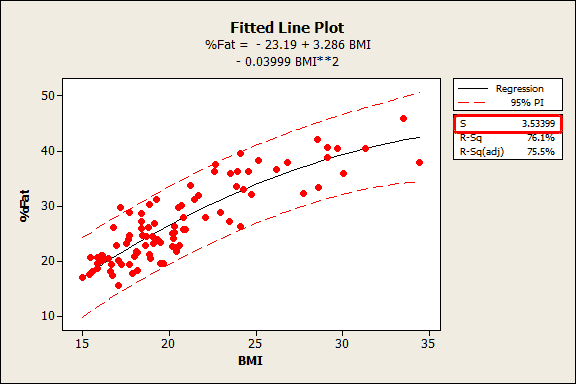
The standard error of multiple linear regression tells us what the average distance between the observed (real values from our data set) and our predicted values from the regression line is. In other words, it basically tells us how bad our overall regression model is on average. This means when we are looking at the standard error a better model will have a lower standard error, while a bad model will have a high standard error.

The standard error of a regression model is sometimes referred to as the standard error of the coefficient estimate. Here is a simple visual of a regression model which has a pretty small standard error.

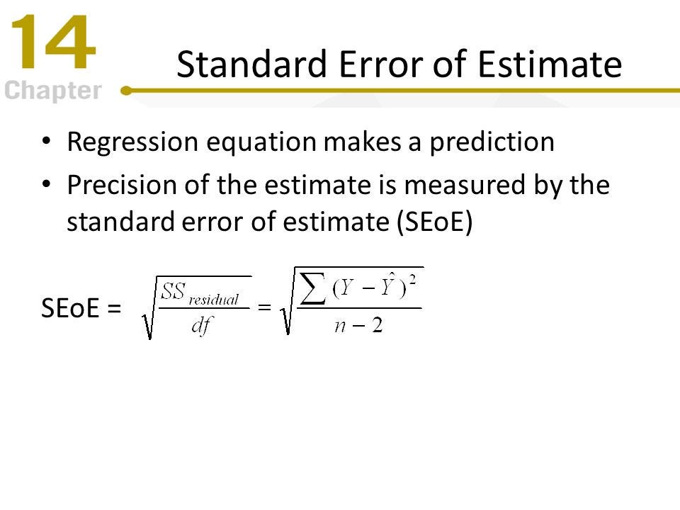
If you want to know the mathematics behind it (the formula) you can view the image below:

Realistically, however, you will probably never have to calculate this by hand.

Degrees of freedom

Complexity vs Performance

Recall from this post, that we saw if we have an extremely large number of columns (parameters), then we can keep feeding our ML model more and more information. The problem is that this would cause our model to start to overfit. However, if we do the opposite, and use the bare minimum, then our model would end up underfitting. So, our job would be to try and find the middle ground here.

So, given this information, how would we figure out mathematically how many columns to keep and how many to discard? To solve this problem, we use something called degrees of freedom.

Degrees of Freedom

Degrees of freedom means the number of parameters (predictor variables) in the model. For linear regression models this would refer to the number of columns, however for tree based models this would refer to things like the tree depth, and for neural networks, this would refer to the number of weights.

Degrees of freedom (df or dof) represents the number of points in a model that can be controlled, which would end up influencing the overall model. In regression analysis, the formula is: degrees of freedom = number of independent values (samples) - number of statistics.

You can use this simple bullet list to get an idea of how the math checks out.

• if we are just dealing with just the mean (this would be just B0), then number of statistics = 1.

• If we are dealing with a simple linear regression (this would be just B0 and B1), the number of statistics = 2.

• and so on...

Put in simple terms, if we have 100 samples, and we have 3 predictor variables, we would have Y=B0+B1+B2+B3 as the regression equation. This means the degrees of freedom we have is 100-4=96. Degrees of freedom are important because you never want to end up with a scenario where you have more independent variable than the number of samples, as this would lead to us getting a negative degrees of freedom, which is an obvious sign of our model overfitting.

Error T Value (test statistic)

The t-test is a statistical test that is used to determine if there is a difference between the means of two groups.

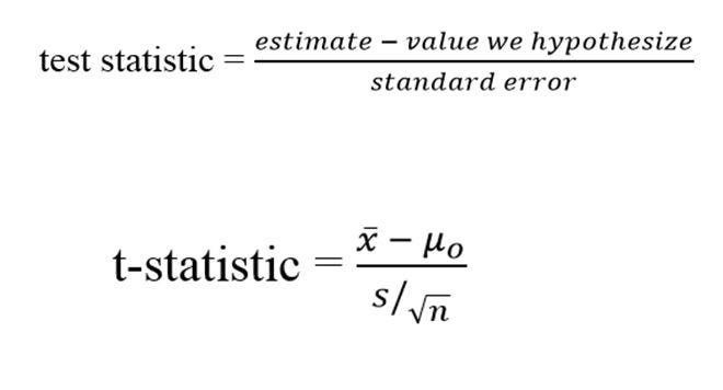
The t-value is calculated by dividing the difference between the means of the two groups by the standard error of those means. This calculation gives you a measure of how likely it is that the difference between the means was due to chance. A large t-value indicates that there is a high likelihood that the difference was not due to chance, while a small t-value indicates that there is a low likelihood that the difference was not due to chance.

P-Value (Statistically significant)

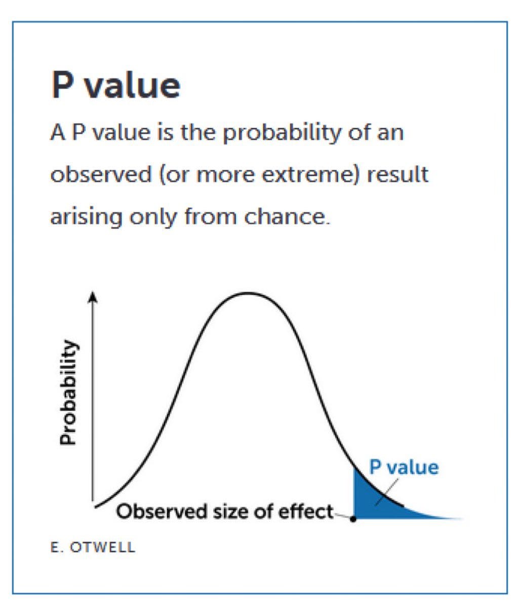
A p-value is a statistical measure that tells you how likely it is that a given result is due to chance. In other words, it tells you how confident you can be in your results.

For example, let's say you're doing a regression analysis to predict teenagers' grades based on their weekly TV-watching habits. After running your analysis, you find that there is a strong relationship between TV-watching and grades (i.e., the more TV younger viewers watch, the lower their grades). The p-value for this relationship would tell you how confident you could be in this result.

Generally speaking, the smaller the p-value, the stronger the evidence against the null hypothesis. Remember, from up above, the null hypothesis says that there is no connection.

In other words, a small p-value tells you that the null hypothesis is false, which indirectly means the alternative hypothesis is correct. This right here is what's called a simple A/B test, and it is used extremely commonly to figure out if a prediction was correct due to just simple random chance, or if there was actually some legit weight behind it. The p-value also relies on a probability distribution called the Chi-Squared distribution.

TLDR: A p-value less than 0.05 typically tells you that there is indeed some strong linear relationship between the explanatory and predictor variables in the same data.

4. Anova model (More Theory)

Anova Tables in General

Remember, ANOVA is a statistical technique used to compare the means of two or more groups. This can be helpful in determining whether the means of the groups are statistically different from each other.

The ANOVA table is a summary of the results of the ANOVA test. This table displays information such as the F-statistic (a measure of how significant the difference between the means is), as well as the p-value (a measure of how likely it is that this difference occurred by chance).

The ANOVA table has three columns. The first column is the name of the variable. The second column is the mean of the variable. The third column is the variance of the variable. This value is calculated by taking the sum of squares and dividing it by the number of observations in the group. Here is an example of an ANOVA table:

I like this example because they also show you a bit of how the other numbers in the F table were constructed.

ANOVA Formulas:

As stated earlier, you typically do not have to do these calculations by hand. But, for those of you who are mathematically inclined, you can look at this simple table here which illustrates the formulas.

F Test

The F-test, otherwise known as the F statistic, or the F-test statistic is a measure of the statistical significance of the difference between two population variances. The F-test statistic is used in the analysis of variance (anova), which is a technique for testing whether the means of more than two groups are equal. The F statistic is computed from the ratio of two variances, and is distributed as an F-distribution under the null hypothesis that all population means are equal.

The F statistic can be used to test the significance of a regression coefficient, or to test whether there is a significant difference between the group means in a one-way or two-way anova.

For those interested, here is what the F distribution looks like visually:

One way anova model

A one way anova test is a statistical method used to test the hypothesis that there is a difference between the means of two or more groups. The ANOVA test compares the variability of the groups' data with the variability within each group. If there is a significant difference between the means, then ANOVA will identify which groups are different.

BowTied_Raptor | Data Science Emporium @BowTied_Raptor

In a One way ANOVA, you have 1 x column, and 1 y column. But, this 1 x column contains categorical data. The idea with 1 way ANOVA is to see there is any actual difference between these said categorical data, or do they all essentially produce the same results.

A one-way anova can be used when you have one independent variable (the factor being tested) and two or more groups. For example, you might want to compare the average weight loss for three different diet plans. In this case, the independent variable would be the type of diet plan (low calorie, low carbohydrate, or moderate calorie/moderate carbohydrate), and the dependent variable would be weight loss.

Here is a pretty video that illustrates what a one way anova test is.

Two Way anova model (Factorial anova)

A two way anova test is an extension of the one way anova test, which can be used to compare more than two groups. The two-way ANOVA allows you to test the difference between two groups at a time, as well as how the different groups interact with each other. The calculation for a two-way ANOVA is more complicated than for a one-way ANOVA, but the basic idea is the same.

BowTied_Raptor | Data Science Emporium @BowTied_Raptor

In a Two way ANOVA, you have multiple x columns, but the premise is the same, you will end up evaluating every single categorical data in the first x column, then evaluate every categorical data in the second x column, and also see if there is any interaction between them.

Here's an example: let's say you want to know if the difference in math test scores between boys and girls is due to sex or age. You would use a two way ANOVA test. The first factor (sex) would be the independent variable and the second factor (age) would be another independent variable, the math test scores themselves would be the dependent variable. Below is the equation for it.

One way vs two way anova model

So, now that we know what a one way and a two way anova variance table is, how do we figure out which one to use for our problem?

There are a few considerations when deciding whether to use a one-way or two-way anova variance table. The first is the number of independent variables. If there is only one independent variable, then a one-way is appropriate. If there are two or more independent variables, then a two-way ANOVA is necessary.

Another consideration is the type of data. If the data are interval or ratio level, then a one-way or two-way ANOVA can be used. However, if the data are ordinal level, then only a one-way can be used. The final consideration is the research design. If the research design is completely randomized, then either a one or a two way anova test.

Here is a concrete example to help out

In the above example, if you only have 1 explanatory variable, but this variable can have a use give multiple different answers: 2,4,6,8, then you will want to go with a one way table. If you have two or more explanatory variables, and like the above example, the user can enter in multiple different answers: ie the levels of hours of training, and their gender, then you will want to go with a two way anova.

Remember, when we say explanatory variable here, we are referring to a categorical variable. You can't have an answer like 2, 4, 6, or 8 if it isn't a categorical variable.

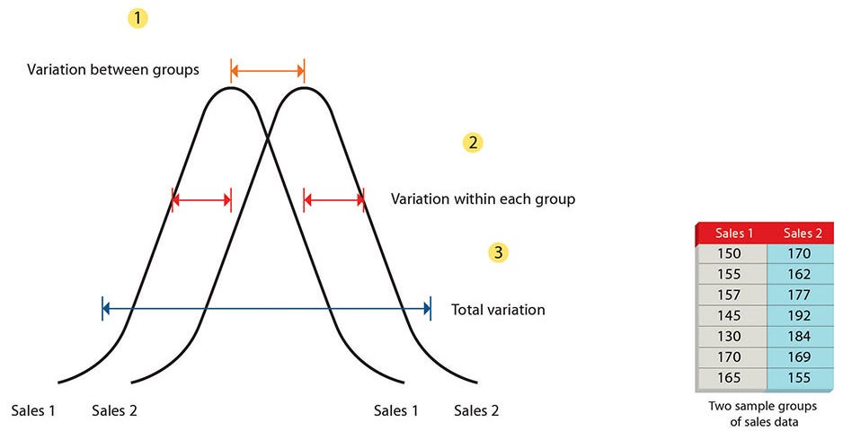
Total Variance

If you were getting confused on what we mean we talk about variability within groups, and variability among groups, here is a simple chart that can help illustrate what we mean.

5. Square Error

Sum of squares (SS) & Mean square error (MSE)

Sum of squares (SS) is a calculation for assessing the difference between the means of more than two groups. The sum of squares measures the variability within each group, and the larger the sum of squares, the greater the variability within that group

The SS calculation considers the differences between all pairs of data points within each group, and then sums these differences together. This sum is then divided by the number of groups, which gives us the mean square error (MS). The MS can be used to determine whether there is a significant difference between the groups, by comparing it to the null hypothesis.

Total sum of errors

The total sum of errors is the sum of the squared difference between each observation and the mean. This quantity is used to calculate the variance and standard deviation of a data set. This is basically just the overall variance for the data, that's it. But, the idea with this is that we can take the variance in the residual, and add it up with the variance from our model above, and they would add up together to get the total sum of errors.

Note: For this picture below, when they say explained sum of squares (ESS), they basically just mean the sum of squares from above (SS).

Note: When we say residual standard error here, it's same residual you would have encountered if you asked R/Python to make a simple residual plot. It's basically a plot on the errors.