Bag of words vs sequence modelling

Comparing the 2 approaches above in a NLP task with deep learning

Historically, most early applications of machine learning to NLP just involved bag-of-words models. Interest in sequence models only started rising in 2015, with the rebirth of recurrent neural networks. Today, both approaches remain relevant. Let’s see how they work, and when to leverage which. We’ll be focusing on 2 approaches in this post.

Bag of words (n-gram), and sequence model.

Prepping the IMDB movie reviews data

Let’s start by downloading the dataset from the Stanford page of Andrew Maas

You can download it from this link: https://ai.stanford.edu/~amaas/data/sentiment/

Once you have it downloaded, go ahead and extract it.

You’ll have 2 folders: train, and test, representing the training and the test data set. Each will have a “pos”, and a “neg” folder, representing the positive, and the negative sentiment data.

Now that we got the data, we’ll want to do a quick train/validation split on 20% of our training data. The code below basically takes some files from our train dataset, and chucks them into a new folder called “val”, and makes this our validation data.

import os, pathlib, shutil, random

base_dir = pathlib.Path(’aclImdb’)
val_dir = base_dir / “val”
train_dir = base_dir / “train”
for category in (”neg”, “pos”):
    os.makedirs(val_dir / category)
    files = os.listdir(train_dir / category)
    random.Random(117).shuffle(files)
    num_val_samples = int(0.2 * len(files))
    val_files = files[-num_val_samples:]
    for fname in val_files:
        shutil.move(train_dir / category / fname,
                    val_dir / category / fname)

Now that we have the train/test/validation folders setup, we can use keras in order to quickly load up the data & their labels. we will use the text_dataset_from_directory to do this.

from tensorflow import keras
batch_size = 32

train_ds = keras.utils.text_dataset_from_directory(’aclImdb/train’, labels=’inferred’,batch_size = batch_size)
val_ds = keras.utils.text_dataset_from_directory(’aclImdb/val’, labels=’inferred’,batch_size = batch_size)
test_ds = keras.utils.text_dataset_from_directory(’aclImdb/test’, labels=’inferred’,batch_size = batch_size)

By using labels = ‘inferred’, keras treats the folder itself as a label, for example all items in the folder “pos” get given the positive label, and all items in the “neg” folder get given the negative label.

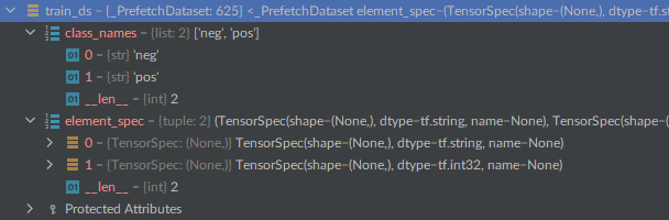
Here’s a quick snapshot of what the data looks like after keras has loaded it for us.

Bag of words approach (N-gram)

Preprocessing our data

The simplest way to encode a piece of text for processing by a machine learning model is to discard order and treat it as a set (bag) of tokens. You could either look at individual words, or try to recover some local order information by looking at groups of consecutive tokens.

If you use a bag of single words, the sentence “the cat sat on the mat” becomes:

{“cat”, “mat”, “on”, “sat”, “the”}

The main advantage of this encoding is that you can represent an entire text as a single vector, where each entry is a presence indicator for a given word. For example, using binary encoding, you’d encode a text as a vector with as many dimensions as there are words in your vocabulary, with 0s almost everywhere and some 1s for dimensions that encode words present in the text.

Let’s go ahead and process our raw text datasets with a TextVectorization layer so that they yield multi-hot encoded binary word vectors. Our layer will only look at single words (unigrams).

from tensorflow.keras.layers import TextVectorization
text_vectorization = TextVectorization(
    max_tokens = 20000,
    output_mode = ‘multi_hot’,
)

text_only_train_ds = train_ds.map(lambda x, y:x)
text_vectorization.adapt(text_only_train_ds)

binary_1gram_train_ds = train_ds.map(
    lambda x, y: (text_vectorization(x), y),
    num_parallel_calls = 4
)
binary_1gram_val_ds = val_ds.map(
    lambda x, y: (text_vectorization(x), y),
    num_parallel_calls = 4
)
binary_1gram_test_ds = test_ds.map(
    lambda x, y: (text_vectorization(x), y),
    num_parallel_calls = 4
)

we set max_tokens to 20,000 to tell keras to limit the vocabulary to the 20,000 most frequent words, otherwise we’d be here all day.

Model-building utility & call

Now let’s write a re-usable model building function that we’ll use in all of our experiments.

Hold onto this section of code below…. we’ll be bringing it up when we compare unigrams, bigrams, etc…

from tensorflow import keras
from tensorflow.keras import layers

def get_model(max_tokens = 20000, hidden_dim = 16):
    inputs = keras.Input(shape = (max_tokens,))
    x = layers.Dense(hidden_dim, activation = ‘relu’)(inputs)
    x = layers.Dropout(0.5)(x)
    outputs = layers.Dense(1, activation = ‘sigmoid’)(x)
    model = keras.Model(inputs, outputs)
    model.compile(optimizer = ‘rmsprop’,
                  loss = ‘binary_crossentropy’,
                  metrics = [’accuracy’])
    return model

now let’s train and test it on our data

model = get_model()
model.summary()
callbacks = [keras.callbacks.ModelCheckpoint(’binary_1gram.keras’, save_best_only = True)]
model.fit(binary_1gram_train_ds.cache(),
          validation_data = binary_1gram_val_ds.cache(),
          epochs = 10,
          callbacks=callbacks)
model = keras.models.load_model(’binary_1gram.keras’)
print(f”Test acc: {model.evaluate(binary_1gram_test_ds)[1]:.3f}”)

Nice, it gave us 88% accuracy test results.

Now let’s look at the sequence model approach

Sequence model approach

The history of deep learning is that of a move away from manual feature engineering, towards letting model learn their own features from exposure to data alone. What if, instead of manually crafting order-based features, we exposed the model to raw word sequences and let it figure out such features on its own?
This is what sequence models are about.

To implement a sequence model, you’d start by representing your input samples as sequence of integer indices. Then, you’d map each integer to a vector to obtain vector sequences. Finally, you’d feed these sequences of vectors into a stack of layers that could cross-correlate features from adjacent vectors.

As of now, bidirectional RNNs are considered the start of the art for sequence modelling

Processing our data

Let’s prepare datasets that return integer sequences.

from tensorflow import keras
batch_size = 32

train_ds = keras.utils.text_dataset_from_directory(’aclImdb/train’, labels=’inferred’,batch_size = batch_size)
val_ds = keras.utils.text_dataset_from_directory(’aclImdb/val’, labels=’inferred’,batch_size = batch_size)
test_ds = keras.utils.text_dataset_from_directory(’aclImdb/test’, labels=’inferred’,batch_size = batch_size)


from tensorflow.keras.layers import TextVectorization
max_length = 600
max_tokens = 20000
text_vectorization = TextVectorization(
    max_tokens = max_tokens,
    output_mode = ‘int’,
    output_sequence_length = max_length,
)

text_only_train_ds = train_ds.map(lambda x, y:x)
text_vectorization.adapt(text_only_train_ds)

int_train_ds = train_ds.map(
    lambda x, y: (text_vectorization(x), y),
    num_parallel_calls = 4)
int_val_ds = val_ds.map(
    lambda x, y: (text_vectorization(x), y),
    num_parallel_calls = 4
)
int_test_ds = test_ds.map(
    lambda x, y: (text_vectorization(x), y),
    num_parallel_calls = 4
)

Most of this code is re-used from the above section, just in case someone wanted to jump directly here and focus on this one first.

Making a model

Great, now, let’s make a model. The simplest way to convert our integer sequences to vector sequences is to one-hot encode he integers (each dimension would represent 1 possible term in the vocabulary). On top of these one-hot vectors, we’ll add a simple bi-directional LSTM.

from tensorflow import keras
from tensorflow.keras import layers

max_tokens = 20000
embed_dim  = 128

inputs = keras.Input(shape=(None,), dtype=”int32”)
x = layers.Embedding(max_tokens, embed_dim, mask_zero=True)(inputs)
x = layers.Bidirectional(layers.LSTM(32))(x)
x = layers.Dropout(0.5)(x)
outputs = layers.Dense(1, activation=”sigmoid”)(x)
model = keras.Model(inputs, outputs)
model.compile(optimizer = ‘rmsprop’,
              loss = ‘binary_crossentropy’,
              metrics=[’accuracy’])
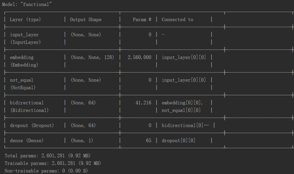
model.summary()

And here’s the model summary:

Calling our model on our data & observations

Now let’s call it on our data

callbacks=[keras.callbacks.ModelCheckpoint(’one_hot_bidir_lstm.keras’, save_best_only=True)]
model.fit(int_train_ds,validation_data=int_val_ds, epochs=10, callbacks=callbacks)
model=keras.models.load_model(’one_hot_bidir_lstm.keras’)
print(f”Test acc: {model.evalate(int_test_ds)[1]:.3f}”)

And this gives us a 86 % on the test set.

The first thing you’ll notice is going with the model sequence approach takes a very, very long time compared to the bag of words approach. This is because our inputs are quite large. Each sample is ended into a matrix of size [600, 20000]. 600 words per sample, out of 20,000 possible words. that’s about 12 MILL values…. per single sample.

And on top of that, we have a bi-direction RNN, so it goes both forwards and backwards which also adds in a crap ton of complexity, hence the increased computation time. And, even with all of that extra information, the model doesn’t perform as well as our bag of words approach.

So, in conclusion converting words to vectors using a 1-hot encoding approach doesn’t work so well….. luckily there is something that does, it’s called “Word Embedding”