Computer Vision on a small dataset

Basically computer vision in the real world

Having to train an image-classification model using very little data is a common situation, which you’ll likely encounter in practice if you ever do computer vision in a professional context. A “few” samples can mean anywhere from a few hundred to a few tens of thousands of images. As a practical example, we’ll focus on classifying images as dogs or cats in a dataset containing 5,000 pictures of cats & dogs. We’ll use 2,000 pictures for training, 1,000 for validation, and 2,000 for testing.

We’ll start off by naively training a small conv-net on the training samples, without any regularization. This will set a base of what can be achieved. Then we’ll start introducing a few other techniques that you can use when faced with this problem.

Relevance of deep learning for small-data problems

What qualifies as “enough samples” to train a model is relative, relative to the size and depth of the model you’re trying to train. For example, it isn’t possible to train a convent to solve a complex problem with just a few tens of samples, but a few hundred can potentially suffice if the model is small, and well regularized and the task is simple.

Deep Learning models are by nature highly re-purposable: you can take an image-classification model trained on a large-scale data-set and reuse it on a significantly different problem with only minor changes. In the case of computer vision, many pretrained models are now publicly available for download and can be used to bootstrap powerful vision models out of very little data. You can use the link below to download & play around with some of them.

https://github.com/balavenkatesh3322/CV-pretrained-model

Preparing our data

The dogs vs cats dataset that we will use for this post is available here: Microsoft-Cats-Dogs-Data

Here’s a few photos of what the data looks like:

As you can see, they are colored photos, each with different dimensions. Some of them are crystal clear photos, others are extremely blurry with bad lighting.

Now, to make this exercise realistic, we’ll go ahead, and we’ll reduce our training data to be 1,000 cat/dog pictures, and have 500 cat/dog pictures.

We’ll also make 2 folders called train, and validation for our separation. Here’s a photo of what my directory looks like.

Building the model

We’ll re-use the model from the previous computer vision post that you saw, but with minor alterations. Since we are dealing with bigger images, and a more complex problem, we’ll make our model larger, so it will have 2 more Conv2D and MaxPooling2D stages. The purpose of these is to augment the capacity of the model, and to further reduce the size of the feature maps so they aren’t overly large when we reach the Flatten layer.

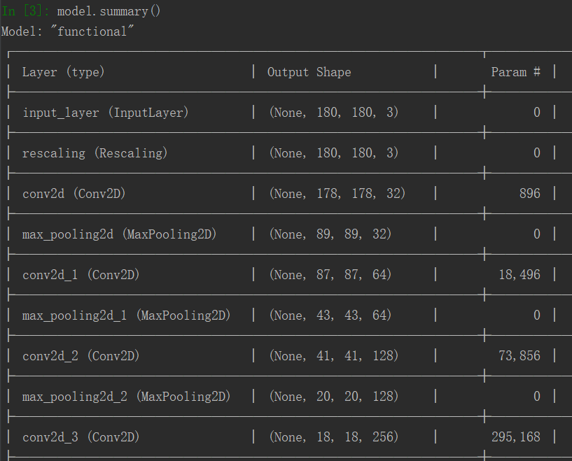
For the sake of simplicity, we’ll resize the dimensions of all the pics to be 180x180, and thus use that for our input size. So, here’s what the model looks like:

from tensorflow import keras
from tensorflow.keras import layers

inputs=keras.Input(shape=(180,180,3))
x=layers.Rescaling(1./255)(inputs)
x=layers.Conv2D(filters=32,kernel_size=3,activation='relu')(x)
x=layers.MaxPooling2D(pool_size=2)(x)
x=layers.Conv2D(filters=64,kernel_size=3,activation='relu')(x)
x=layers.MaxPooling2D(pool_size=2)(x)
x=layers.Conv2D(filters=128,kernel_size=3,activation='relu')(x)
x=layers.MaxPooling2D(pool_size=2)(x)
x=layers.Conv2D(filters=256,kernel_size=3,activation='relu')(x)
x=layers.MaxPooling2D(pool_size=2)(x)
x=layers.Conv2D(filters=256,kernel_size=3,activation='relu')(x)
x=layers.Flatten()(x)
outputs=layers.Dense(1,activation='sigmoid')(x)
model=keras.Model(inputs=inputs, outputs=outputs)

And here is what the model summary looks like:

RMSprop optimizer is generally good for image tasks, so we’ll stick with that. And, for the loss, since we are dealing with a single sigmoid unit, we’ll use the binary crossentropy, since it’s a binary classification problem.

model.compile(loss='binary_crossentropy',
              optimizer='rmsprop',
              metrics=['accuracy'])

Data preprocessing

As you know by now, data should be formatted into appropriately preprocessed floating point tensors before being fed into the model. Currently, the data sits on your hard drive as JPEG files, so the steps for getting it into the model are roughly as follows:

1. Read the picture files.

2. Decode the JPEG content to RGB grids of pixels.

3. Convert these into floating-point tensors.

4. Resize them to a shared size (in our case 180x180)

5. Pack them into batches (we’ll use batch size of 32).

Coding all of this from scratch is a painful process, luckily Keras pretty much already has these functions ready for us, and all we need to do is point them to the data. Here’s the code for it:

from tensorflow.keras.utils import image_dataset_from_directory
train_dataset=image_dataset_from_directory(
    'train',
    image_size=(180,180),
    batch_size=32)
validation_dataset=image_dataset_from_directory(
    'validation',
    image_size=(180,180),
    batch_size=32)

Model training & assessment

Let’s fit our model on our dataset, and then take a look at the performance.

Here’s the code for fitting the model

callbacks = [
    keras.callbacks.ModelCheckpoint(
        filepath='convnet_low_data.keras',
        save_best_only=True,
        monitor='val_loss'
    )
]
history=model.fit(
    train_dataset,
    epochs=30,
    validation_data=validation_dataset,
    callbacks=callbacks
)

If we look at the last few epochs we can see that the validation accuracy hovers around 70-75%, while the training accuracy goes to like almost 100%. Clearly, this model is overfitting, so… sounds like we’ll have to solve this problem.

Using Data Augmentation

Overfitting is caused by having too few samples to learn from, rendering you unable to train a model that can generalize to new data. Given infinite data, your model would be exposed to every possible aspect of the data distribution at hand: you would never overfit.

Data augmentation takes the approach of generating more training data from existing training samples by augmenting the samples via a number of random transformations that yield believable-looking images. This helps expose the model to more aspects of the data so that it can generalize better.

Luckily, keras lets us a way to quickly do this.

data_augmentation = keras.Sequential(
    [
        keras.layers.RandomFlip('horizontal'),
        keras.layers.RandomRotation(0.1),
        keras.RandomZoom(0.2)
    ]
)

From above, the RandomFlip applies a horizontal flip. Random Rotation rotates the photo +/- 10 degrees. The Random Zoom zooms in/out of the image by +/- 20%.

If you want to see a list of all possible augmentations, you can visit this link here.

Now that we have this done, here’s a preview of what the augmented photos looks like.

Training a new model with data augmentation

Now that we have data augmentation done. Another thing we can do is implement dropout near the end so that it shuts off a lot of the parameters randomely, which will help us solve our overfitting problem. Here’s the code for that.

inputs=keras.Input(shape=(180,180,3))
x=data_augmentation(inputs)
x=layers.Rescaling(1./255)(inputs)
x=layers.Conv2D(filters=32,kernel_size=3,activation='relu')(x)
x=layers.MaxPooling2D(pool_size=2)(x)
x=layers.Conv2D(filters=64,kernel_size=3,activation='relu')(x)
x=layers.MaxPooling2D(pool_size=2)(x)
x=layers.Conv2D(filters=128,kernel_size=3,activation='relu')(x)
x=layers.MaxPooling2D(pool_size=2)(x)
x=layers.Conv2D(filters=256,kernel_size=3,activation='relu')(x)
x=layers.MaxPooling2D(pool_size=2)(x)
x=layers.Conv2D(filters=256,kernel_size=3,activation='relu')(x)
x=layers.Flatten()(x)
x=layers.Dropout(0.5)(x)
outputs=layers.Dense(1,activation='sigmoid')(x)
model=keras.Model(inputs=inputs, outputs=outputs)

model.compile(loss='binary_crossentropy',
              optimizer='rmsprop',
              metrics=['accuracy'])

And, here’s how you can train the model

callbacks = [
    keras.callbacks.ModelCheckpoint(
        filepath='convnet_low_data.keras',
        save_best_only=True,
        monitor='val_loss'
    )
]
history=model.fit(
    train_dataset,
    epochs=50,
    validation_data=validation_dataset,
    callbacks=callbacks
)

And, now you can see the performance of our new model went to 75 to 80%. That’s a bump in 5% with absolutely no extra data.