Deep Learning 10 - Computer Vision

Your First computer vision model

Computer vision is the earliest success story of deep learning. Computer vision is the problem domain that led to the initial rise of deep learning between 2011 and 2015. A type of deep learning model called convolutional neural networks started getting remarkably good results on image classification competitions around that time.

1 - Intro to convnets

In this link, we made a fully connect dense neural network (Multi layered perceptron) to classify the MNIST digits. We are going to discuss how a convnet works, then, by the end of the post, we’ll build a simple convnet, that will tackle the exact same problem as our dense neural network above, and you can see the difference in performance right there.

The fundamental difference between a densely connected layer and a convolutional layer is this:

• Dense layers learn global patterns in their input feature space (ie for MNIST digit, patterns involving ALL pixels)

• Convolutional layers learn local patterns - in the case of images, patterns found in small 2D windows of the inputs (see example below)

This key characteristic gives convents 2 interesting properties

1. The patterns they learn are translation-invariant. After learning a certain pattern in the lower right corner of a picture, a convent can recognize it anywhere: for example in the upper left corner. This makes convents data-efficient when processing images, which means they dont need as many training samples to learn

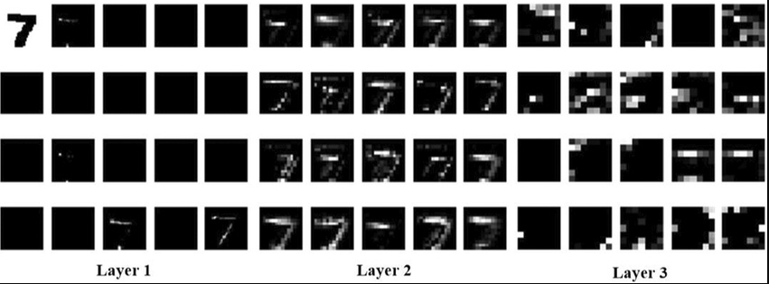
2. They can learn spatial hierarchies of patterns. A first convolutional layer will learn small local patterns such as edges, a second convolutional layer will learn larger patterns made of the features of the first layers, and so on….

2 - Feature maps

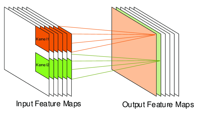
Convolutions operate over rank-3 tensors called feature maps, with 2 spatial axes (height, width, and depth). The depth axis is sometimes called the “channels” axis.

For an RGB image, the depth axis is 3 because it has 3 color channels:

• Red

• Green

• Blue

For a black, and white pictures (like the MNIST digits data above), the depth is 1 (levels of grey). The convolution operation extracts patches from its input feature map and applies the same transformation to all of these patches, producing an output feature map.

This output feature map is still a rank