Deep Learning 5: Classifying Reuters' newswires

Information Bottleneck, and Multiclass classification problem for the thomas reuters' newswires dataset

Last section, we did a binary classification problem, this time, we’ll do a multi class classification problem. In this one, we’ll build a deep neural network to classify Reuters newswires into 46 mutually exclusive topics. Because I said they are mutually exclusive topics, we are dealing with a single-label multiclass classification problem.

Sometimes, in the real world, you’ll encounter a scenario where a data point could belong to multiple classes at the same time. Those are called multilabel multiclass classification problems.

We’ll also cover information bottleneck. A real problem many of you will encounter in the real world.

1 - Load up the dataset

To load up the dataset, we’ll use the following code:

from tensorflow.keras.datasets import reuters
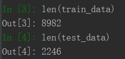
(train_data, train_lables), (test_data, test_labels)=reuters.load_data(num_words=10000)

Just like with the IMDB dataset, by saying num_words, we restrict the data to only deal with the top 10,000 most frequently used words. We can use the len() function to see how many samples we have in the training & the test data:

If we try to take a look at the data, we’ll see it’s just a bunch of numbers. Just like with the IMDB dataset, each number is pointing to a specific word on a mapped dictionary:

1.1 Decoding the data

To decode the data, we’ll use the get_word_index() function from the reuters module. Then, just write a simple reverse dictionary code to do so.

word_index=reuters.get_word_index()
reverse_word_index = dict(
    [(value, key) for (key, value) in word_index.items()]
)
decoded_newswire = " ".join(
    [reverse_word_index.get(i-3," ") for i in train_data[0]]
)

And here’s what the decoded_newswire says:

2 - Preparing the data

Just like how we did the encoding in the IMDB dataset, we’ll have to encode this data as well. To do this, we’ll just call upon our old vectorize_sequences function.
If you lost it, here’s the code below for it:

import numpy as np
def vectorize_sequences(sequences, dimension=10000):
    results = np.zeros((len(sequences), dimension))
    for i, sequence in enumerate(sequences):
        for j in sequence:
            results[i, j] = 1
    return results

And, then point your train & test data to it:

X_train = vectorize_sequences(train_data)
X_test = vectorize_sequences(test_data)

Now that we got the X data vectorized, we’ll want to also encode the labels. More specifically we’ll want to do one hot encoding. Here’s an image of what it looks like:

Luckily Keras already has an inbuilt function for this (to_categorical), so we just call it:

from tensorflow.keras.utils import to_categorical
Y_train = to_categorical(train_lables)
Y_test = to_categorical(test_labels)

3 - Building Your Model

This classification problem looks similar to the previous movie review classification problem. In both cases, we are trying to classify short snippets of text. But there is a new constraint here: the number of output classes has gone from 2 to 46. In other words the dimensionality of the output space is much larger.

In a stack of DENSE layers, each layer can only access information present in the output of the previous layer. If one layer drops some information relevant to the classification problem, this information can never be recovered by later layers: each layer can potentially become an information bottle neck.

In the previous example, we used 16 dimensional intermediate layers, but a 16D space may be too limited to learn to separate the 46 different classes. Such small layers may act as information bottlenecks, permanently dropping relevant information. So, because of this reason, we’ll go with layer layers. Let’s do 16.

model = keras.Sequential([
    keras.layers.Dense(64,activation='relu'),
    keras.layers.Dense(64,activation='relu'),
    keras.layers.Dense(46,activation='softmax')
])

Since we have 46 classes to predict from, the final number of perceptrons (units) in our final layer = 46.

Because we are dealing with a multiclass classification problem, we’ll also use the categorical cross-entropy loss function

model.compile(optimizer='rmsprop',
              loss='categorical_crossentropy',
              metrics=['accuracy'])

4 - Validation, Train & Test

Let’s seperate out about 1000 samples, and make that our validation set.

X_val=X_train[:1000]
partial_X_train=X_train[1000:]
Y_val=Y_train[:1000]
partial_Y_train=Y_train[1000:]

Now, let’s begin the training process

history=model.fit(partial_X_train,
                  partial_Y_train,
                  epochs=20,
                  batch_size=512,
                  validation_data=(X_val,Y_val))

And, here’s the training process visualized:

While we are at it, let’s go ahead and plot the training accuracy with the validation accuracy so we can see them side by side:

from matplotlib import pyplot as plt
plt.clf()
acc=history.history['accuracy']
val_acc=history.history['val_accuracy']
loss=history.history['loss']
epochs=range(1,len(loss)+1)
plt.plot(epochs,acc,"bo",label='training acc')
plt.plot(epochs,val_acc,"b",label='validation acc')
plt.xlabel('epochs')
plt.ylabel('accuracy')
plt.title('training & validation acc')
plt.show()

Anyways, once you’ve loaded up the graph, you’ll see that the model starts to overfit around epoch 10.

5 - Retraining, and evaluation

Cool, let’s go ahead and retrain our model above, and set the epochs to 10.

history=model.fit(partial_X_train,
                  partial_Y_train,
                  epochs=10,
                  batch_size=512,
                  validation_data=(X_val,Y_val))

And to evaluate our model, we’ll just use the .evalute() method. Here’s what it looks like:

Cool, seems like we got a 78% of Out sample accuracy.

Recall, up above I mentioned if you reduce the number of units drastically, there’s a chance that the next layer may not get sufficient amount of information.

So, let’s test that.

6 - Information Bottleneck

Let’s go with a (64, 2, 46) Densely connected neural network:

model = keras.Sequential([
    keras.layers.Dense(64,activation='relu'),
    keras.layers.Dense(2,activation='relu'),
    keras.layers.Dense(46,activation='softmax')
])

model.compile(optimizer='rmsprop',
              loss='categorical_crossentropy',
              metrics=['accuracy'])
history=model.fit(partial_X_train,
                  partial_Y_train,
                  epochs=10,
                  batch_size=512,
                  validation_data=(X_val,Y_val))

Great, now let’s run the exact same model.evaluate() above, and see the new training & validation accuracies.

Wow… amazing, a 37% accuracy. And this…. is the perfect demonstration of information bottleneck. You’ll always want more units rather than less.