Deep Learning 6: Predicting House prices

The previous 2 examples we did were classification problems, where the goal was to predict a single discrete label of an input data point. Another common type of a machine learning problem you’ll have to face is called regression, it consists of predicting a continuous value instead of a discrete label.

Note: Do not confuse regression and logistic regression. Logistic regression is not a regression algorithm, it’s a classification algorithm.

For this post, we’ll try to predict the median price of homes in a Boston suburb, in the 1970s.
We’ll be given plenty of data regarding things like:

• Crime Rate

• Local Property Tax

• House size

• Number of rooms

• etc…

In the previous 2 posts, we had a lot of samples, and minimal number of Independent variables. In other words, we had lots of rows, but minimal number of X columns.

In this case, it’ll be the opposite, we’ll have a relatively few data points, and lots of X columns.

1 - Load up the data

You can load up the data using the following code:

from tensorflow.keras.datasets import boston_housing
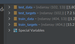
(train_data, train_targets),(test_data, test_targets) = (boston_housing.load_data())

Here are the dimensions of our data:

Here’s a small preview of the training_data:

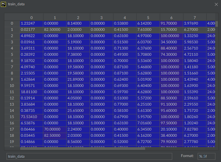
And, here’s the mapping of what each column means:

2 - Preparing Your data

It would be a problem to feed into a neural network, values that all take wildly different ranges. It is possible that the model might be able to automatically adapt to such heterogeneous data, but it would definitely make learning more difficult. A good approach to tackling this would be to do a feature-wise normalization: for each feature in the input data, we subtract the mean of the feature and divide by the standard deviation, so that the feature is centered around 0 and has a unit standard deviation.
Here’s the code for it:

mean = train_data.mean(axis=0)
train_data-=mean
std_dev=train_data.std(axis=0)
train_data/=std_dev
test_data-=mean
test_data/=std_dev

Here’s the before and after of how the values change:

Before:

After:

3 - Building Your model

Because we have so few samples available, we’ll have to use a very small model with 2 intermediate layers, each with 64 units (perceptron). In general, the less training data you have, the worse overfitting will be, and using a small model is one way to mitigate overfitting

Here’s the code:

def my_model():
    model=keras.Sequential([
        keras.layers.Dense(64,activation='relu'),
        keras.layers.Dense(64, activation='relu'),
        keras.layers.Dense(1, activation='relu')
    ])
    model.compile(optimizer='rmsprop',loss='mse',metrics=['mae'])
    return model

Because we need to instantiate the same model multiple times, we are using a function to construct it. This model ends with a single unit, and no activation (this means it will be a linear layer). This is a typical setup for a scalar regression.

Scalar regression is a type of regression where you’re trying to predict a single continuous value. Applying an activation function would constrain the range the output can take; for example, if you applied a sigmoid activation function to the last layer, the model could only learn to predict values between 0 and 1. Here, because the last layer is purely linear, the model is free to learn to predict values in any range.

4 - Validation using k-fold

To evaluate our model, while we keep adjusting it’s parameters, we could split the data into a training set and a validation set, just like we did in the last example. But…. because we have so few data points, the validation set would end up being stupidly small. So…. what we’ll do is implement the k-fold cross validation.
Image below sums it up

In our case, we’ll run a 4 fold cross validation. let’s start building the foundation of the for loop:

k=4
num_val_samples = len(train_data) // k
num_epochs = 100
all_scores = []
for i in range (k):

Now, let’s prepare the validation data, and the training data. Code for it below (keep in mind this runs inside the for loop):

    print(f'proceessing fold number: {i}')
    val_data=train_data[i * num_val_samples: (i+1) * num_val_samples]
    val_targets = train_targets[i * num_val_samples: (i+1) * num_val_samples]

    partial_train_data=np.concatenate(
        [train_data[:i * num_val_samples],
         train_data[(i+1) * num_val_samples:]], axis=0
    )

    partial_train_targets = np.concatenate(
        [train_targets[:i * num_val_samples],
         train_targets[(i+1) * num_val_samples:]], axis=0
    )

And now, let’s send this to the Keras model, and train it

    model = my_model()
    model.fit(partial_train_data,partial_train_targets,
              epochs=num_epochs,batch_size=16,verbose=0)

And don’t forget to track the evaluation on the validation data.

    val_mse,val_mae=model.evaluate(val_data,val_targets,verbose=0)
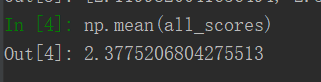
    all_scores.append(val_mae)

And, here is our validation errors:

Seems like in general we tend to have scores between 2.1 and 2.6, and the avg being 2.4

What we’ll want to do next is try and figure out what we want to set the num of epochs to, so that we don’t end up overfitting the neural network.

5 - Final Touches

Let’s go ahead and start saving the validation logs at each fold. So take the above for loop we made earlier, and make some minor tweaks

k=4
num_val_samples = len(train_data) // k
num_epochs = 500
all_scores = []
all_mae_histories=[]
for i in range (k):
    print(f'proceessing fold number: {i}')
    val_data=train_data[i * num_val_samples: (i+1) * num_val_samples]
    val_targets = train_targets[i * num_val_samples: (i+1) * num_val_samples]
    
    partial_train_data=np.concatenate(
        [train_data[:i * num_val_samples],
         train_data[(i+1) * num_val_samples:]], axis=0
    )

    partial_train_targets = np.concatenate(
        [train_targets[:i * num_val_samples],
         train_targets[(i+1) * num_val_samples:]], axis=0
    )

    model = my_model()
    history = model.fit(partial_train_data,partial_train_targets,
                        validation_data=(val_data, val_targets),
                        epochs = num_epochs,batch_size=16,verbose=0)
    mae_history=history.history['val_mae']
    all_mae_histories.append(mae_history)

once we got the above data, we’ll want to fetch the avg of the mae histories

average_mae_history = [np.mean([x[i] for x in all_mae_histories]) for i in range(num_epochs)]

Let’s go plot this bad boi

plt.plot(range(1, len(average_mae_history) + 1), average_mae_history)
plt.xlabel('epochs')
plt.ylabel('validation mae')
plt.show()

great, the graph looks ugly as sin, let’s zoom in, by getting rid of the first 10 epochs.

oh sweet, seems like if we have the epoch around 130ish, we’ll outperform the initial default we had (epoch of 100)