Stats Analysis 1: The 5 Number Summary & IQR
Introducing the Concept of Stats Analysis, and why you need it, the 5 number summary, and the Inter Quartile Range (outlier detection method)
Table of Contents:
Stats Analysis Introduction
The 5 Number Summary
The Dataset
Outlier Detection
1 - Stats Analysis Introduction
Recall from this post that Data Science (DS) is a merger between computer programming, biz domain knowledge, and maths & stats analysis. With the linear algebra series making decent progress, we can now also start working on basic statistics knowledge as well here. Statistical analysis is the process of analyzing a bunch of data to see some sort of an underlying pattern, or to see if any trends exist (including seasonal effects).
There are 2 main types of stats analysis: Descriptive analysis, and statistical inference
Descriptive Analysis
Descriptive analysis is meant to describe a big chunk of data. To describe the data, we will want to use things like charts, tables, etc… The main difference is we do not intend to analyze the data, and try to draw a conclusion here. All we are interested in, is just a quick skim of the data, and that’s about it.
Statistical Inference
The second type of stats analysis is called statistical inference. In this section, we are interested in actually studying the data, and seeing what type of conclusions we can draw from it. This is where we would also conduct our hypothesis testing (A/B testing), and actually try to build models to try to explain the data.
2 - The 5 Number Summary
The 5 number summary is useful in the preliminary phases when you are analyzing a large dataset. The summary of the 5 values consist of: the min, lower quartile (Q1), median (Q2), upper quartile (Q3), and the maximum. Since these are all numeric calculations, the assumption is the vector that you are using this on is purely numeric data.
These values are great because each of them gives us a bit of a snapshot of what the data looks like. The min and max tells us what the hard boundaries are, and the Q1, median, and Q3 give us an idea of the distribution, are these 3 numbers centered around the median, if so, then the data is mostly around the mean/median. Or, are these values a bit more closer to the max, or the min.
3 - The Dataset
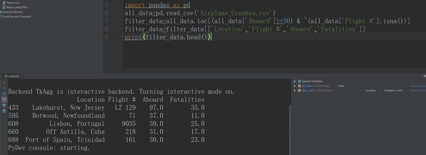
For this little exercise, we’ll use the airplane crashes dataset available here: https://lms.pps.net/courses/14878/files/62768. This dataset has a lot of things in there, that we’ll want to tweak. It has blanks in there (incomplete data). It also has helicopter crashes in there, we don’t care about that. It also has small private airplanes in there as well, we don’t care about that, we want to look at the major airlines that have a lot of passengers for this.
So, we will want to do a simple filter that says only look at the rows
where the aboard >=30. This will make sure we are only look at those that have had a lot of passengers.
We will also make sure the flight # is not blank, that is the flight # is not NA. I’m also going to kick out a lot of the columns, so we have something for a nice quick preview.
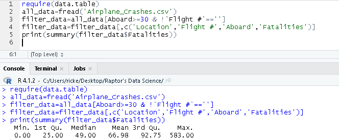
R
Note: although it looks like we should use the is.na() here, unfortunately, that doesn’t work here because once the data is loaded, it actually shows up as an empty string instead of na.
Python
In Python, when it detects a bunch of blanks as entries, it will automatically flag them as nan. NaN means Not a Number, this is pandas’ way of telling us that the entry that is there is blank. In order to deal with this, we will use the .isna() to filter it out.
Note: Another thing to notice is the ~ on line 7. This is because instead of using the not() function, or the ! as in R. In pandas, if you wish to use not for sub setting, you will be using ~ instead. Also, I could change the aboard and fatalities to integers, but meh, it’s fine.
Q0 (Min)
Min is just short for minimum. If we have a set of number, what is the lowest number that exists. Min is good for descriptive stats, because it tells us where our dataset starts from. We can also use min as a quick typo, or crappy data detection. For example, in our current example of examining the fatalities in plane crashes, there is no reason for there to be a negative number in that column.
R
in R, we can just use min() and then navigate to the column of our interest.
Python
In Python, we can just use the min() function on our column of interest.
Q1 (25th Quantile)
The Q1, also called the 25th quantile lets us know where some of our smaller numbers are located. The Q1 is generally a pretty good estimate of skewness. We can take a look at this, and see if it’s closer to the minimum, or closer to the median.
R
In this case, we want to use the quantile() function, and provide it with our column, and also tell it we want the 0.25th value (25% percentile).
Python
For this one, we want to use the .quantile() function provided from the numpy library.
Q2 (Median)
The median of the data tells you where the center of the data is. Median is similar to average because both of them tells you where the center of the data is located. The difference is, unlike an average, the median is much less sensitive to outliers.
R
We can just use the median() function on our data of choice.
Python
The median() from the numpy library can take care of this.
Q3 (75th Quantile)
The Q3, also called the 75th quantile lets us know where some of our larger numbers are located. The Q3 is generally a pretty good estimate of skewness. We can take a look at this, and see if it’s closer to the maximum, or closer to the median.
R
Just the same thing as in the Q1 section.
Python
Just the same thing as in the Q1 section.
Q4 (Max)
This would be the maximum value that exists in our little dataset. This is useful especially for things like outlier detection. Say for example, you were looking at a dataset of gas prices. Instead of typing in $2, and then $3, a person could do a typo and hit $23. This is a pretty quick and easy way of spotting it.
R
We can just use the max() on a vector.
Python
We can just use the max() from the numpy library.
5 Number Summary in R (Easily):
We can actually just straight up use the summary() on a dataset, and R will automatically calculate the 5 number summary for us.
4 - Outlier Detection
Outliers are items in our dataset which go against the norm that the data is telling us. For example, a lot of the Gen Z was practically born with an IPad, and knows how to use a computer really well. However, if you run into a member of Gen Z who says they don’t know how to use a computer, they would be the outlier.
Detecting outliers is extremely important because when we build models on our data, we want to be working with some nice clean, and refined data. Having outliers in there will mess with the calibrations of the statistical models, and give us some extremely wonky conclusions.
Interquartile Range (IQR)
The Interquartile range (IQR) tells us how our data is dispersed. Generally speaking, if we expect most of our numbers to be around 0, and 100…. yet find a random data point at 500, obviously, that 500 is an outlier. In order to come up with the boundaries on how wide our dispersion should be, we rely on this formula:
If we get a value smaller than the lowest value, or a value that’s higher than the highest value from the above calculations, then those values are considered to be outliers.
R
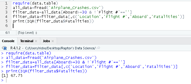
We can just use the IQR() on a dataset to calculate the IQR, from there we can manually calculate the lowest and highest values, and then manually subset our data if we so choose to do so.
Python
We can use the iqr() from the scipy’s library. Just make sure to navigate to it by doing: scipy.stats
For some cool funsies, here is what the histogram of that dataset looked like:


