Log Linear Model
Log Linear model, this is not the same as logistic regression. This one is actually meant for regression analysis, not classification problems.
Table of Contents
Frequently Asked Questions
Implementing a log linear model in R & Python
Linear Model (Regression)
Log Transformation
Independent variables & log linear models
1. Frequently Asked Questions
1.) Why do we use log in linear regression?
The usage of a logarithm in linear regression comes from its ability to 'linearize' the relationship between the independent (X) and dependent (Y) variables. This means that the logarithm of Y corresponds to a linear function of the logarithm of X.
This is important because it enables us to use linear regression to portray the relationship between Y and X, disregarding the non-linear elements in the data. Basically, if we apply a logarithmic transformation to our data, we can safely assume that the relationship between Y and X is linear.
This assumption is important because it lets us leverage standard techniques for modeling linear relationships.
2.) What is the function of a log-linear model?
let’s define linear relationship first. In a linear relationship, you have an A log-linear model is a machine learning model designed to predict the relationship among two or more variables. It’s useful for predicting relationships that are nonlinear (i.e., not a straight line).
The 'linear' in the name means the model's presumption of a linear relationship between the input and output variables. And, 'log' refers to the model's use of a logarithmic transformation of the input data before fitting it into a linear equation. This transformation accommodates nonlinear relationships in the data, resulting in a more accurate prediction of those relationships.
3.) What is the implication of logarithmic data?
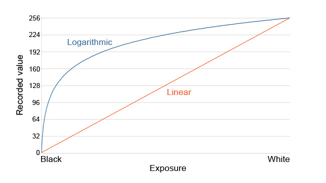
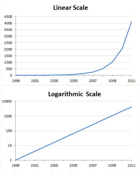
A logarithmic scale is one in which the gap between figures expands or contracts at a proportional rate. If you were to plot the number of Facebook users over time on a linear scale, the line's slope would be steepest in the initial years, then gradually taper as more individuals joined. However, if you plotted the same data on a logarithmic scale, the line's slope would remain approximately constant over time. This is because a logarithmic scale condenses large distances and expands small distances.
In data science, logarithmic data is commonly employed when there's a power law relationship between two variables. Power law essentially means you'll be dealing with exponents, necessitating the use of a logarithmic transformation (or natural log) to make the data functional.
4.) How is a log regression coefficient interpreted?
A log regression coefficient quantifies the relationship's strength between a predictor and an outcome. When the predictor is input into the model as a transformed variable (i.e., in terms of its natural logarithm). It shows how much change in the outcome corresponds to a one-unit shift in the predictor, after adjusting for all other predictors in the model.
The sign of a log regression coefficient reveals the direction of the relationship between the predictor and outcome (either positive or negative), while its magnitude indicates the strength of that relationship. Ideally, your model should have statistically significant log regression coefficients for all your predictors, meaning p-values should be less than 0.05.
5.) What distinguishes linear from logarithmic regression?
Linear regression is a way of describing how one variable (the dependent variable) changes with respect to changes in another variable (the independent variable). In linear regression, the equation expressing the relationship between the two variables is a straight line.
On the other hand, logarithmic regression also illustrates how one variable changes concerning changes in another variable. However, in logarithmic regression, the equation that articulates the relationship between the variables is a curved line. Logarithmic regression is commonly employed when working with data that adheres to a power law
2. Implementing a log linear model in R & Python
For this dataset, we will use the opossum dataset. We'll start off by doing a simple log transformation on our data set. Doing so will transform the residuals from a normal distribution to a lognormal distribution. Once we are done with that, we can just continue and run the simple linear regression model as normal without any trouble.
In this case, what we will do is apply the log fn on our dependent variable (age), then run a simple linear model on it. Then we will run the predictions, and apply an inverse log fn, and then round off the predicted values. Typically, you will want to apply this technique on data where you have exponential growth.
To run the regression in R, we will use the lm() function, to run it in Python, we'll use sklearn's LinearRegression() function.
R
Loading up our data
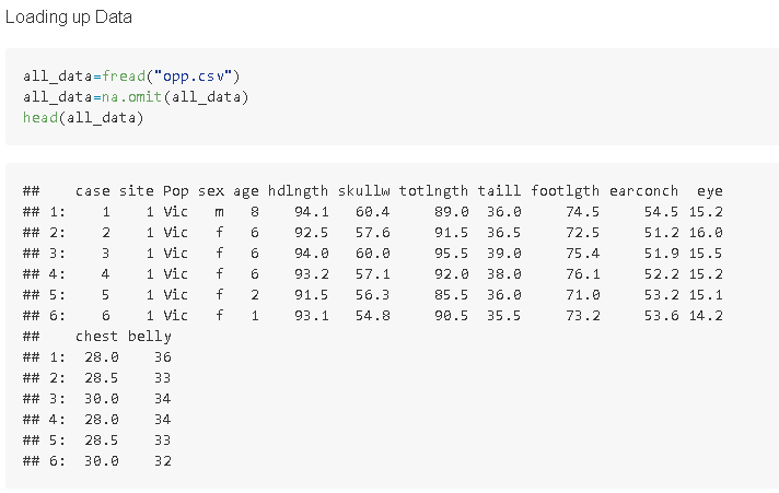
As usual, we'll load up our data using the fread() function from the data.table library. For more information on libraries, click here.
Transforming our data points
With our data read to go, let's do a simple train and test split. Then we'll apply the log fn to our training data set's dependent variable. We will also kick out some useless independent variables.
Running a Log Linear Model
Running the log linear model is basically no different than running a linear regression model in R. Just use the lm() function on your data, just point the dependent and independent variables, and do some model parameters tweaking if you have to.
Predicting and evaluating a log linear model
We just use the predict() function, and point our test data at it, and the job is done. Surprisingly, even though log linear models aren't meant for this type of problem, you can see this one performed quite well.
Python
Loading up our data
we'll use the .read_csv() function from the pandas library to load up the oppossum data set. The goal of the this task is to use a log linear model to try to predict the age of the opossum given a lot of data about the oppossum.
Transforming our data points
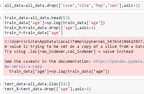
With our data read to go, let's do a simple train and test split. Then we'll apply the log fn to our training data set's dependent variable. We will also kick out some useless independent variables.
Running a Log Linear Model
Now, we will just call upon the LinearRegression() function, and have it fit our Training X data, and our Training Y data.
Predicting and evaluating a log linear model
We just use the predict() function, and point our test data at it, and the job is done. Surprisingly, even though log linear models aren't meant for this type of problem, you can see this one performed quite well.
3. Linear Model (regression)
Recall that Multiple linear regression tries to fit a linear regression model (linear line) for 1 response variable using multiple explanatory variables. Here is the equation it tries to solve for:
Unfortunately, this model has a few limitations. What if you were trying to use this to analyze something that is quadratic, cubic, or some sort of a exponential function? In that case, this current version would fail badly. Here's a few more limitations of a linear model.
Limitations of a linear model
To stick to the top of log linear model, I will only list out the limitations that exist in linear models, but do not exist in the log linear model.
Linear models are only able to extrapolate, while log linear models can also interpolate
Linear models are less accurate when predicting values far outside the input data range
Linear models can not handle non-normalized data that well, hence why we typically have to use some sort of a scaler from sklearn
Each additional predictor increases the complexity of the model by 1 degree, which makes it very very likely to easily overfit. See this post for more information. We used p-value to prove this.
4. Log Transformation
The log transformation means taking a log function, or a ln (natural log fn) if you prefer, and applying this function to our data. When this function is applied to our data, if it was some sort of an exponential distribution, this then converts it to a linear distribution, which we can then go ahead and easily throw in a trend line at. Observe below:
Log Linear Models
In a log linear model, we basically apply the log transformations function to our dependent variables (the y values). Here's a wiki article on some of the mathematics behind it. By doing so, this let's us basically take an exponential distribution, and helps scale the values down to a more workable linear distribution.
In other words, our data should now have some sort of a linear relationship, so any basic linear regression model should be competent enough to get the job done. This process is sometimes referred to as log linear modeling, or a first form log linear model. Here's a visual video to help you out a bit.
Log Linear Model
Now that we've got the theory out of the way, let's talk about more about the impact this model has in data science.
The advantage of using a log linear model is that it can better handle datasets with many predictor variables and/or interactions between predictor variables. The logarithmic transformation helps to "smooth" out the relationships between the variables, making them easier to visualize and interpret.
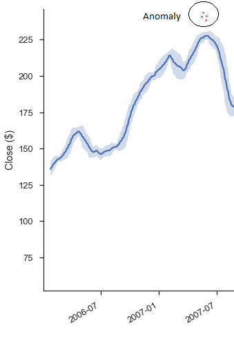
Loglinear models are commonly used in data science and machine learning tasks such as predictive modelling, anomaly detection, and clustering.
The basic thought process is that once you've applied a log transformation upon your dependent variables, you will have effectively smoothened out the curve. But, even after smoothing out the curve to a simple linear model, if you still have weird response variable that is just too far away from what should be considered acceptable, then that thing is clearly an outlier. In such cases, you will typically want to just do whatever your company policy for outlier detection.
5. Independent variables & log linear models
Remember, since you are applying the log transformation scale on your dependent variable (exponential growth), you are effectively re-scaling the y values to bring them more in line to what a linear regression model would be like. In this case, when you look at the coefficients for your independent variables, you have to remember that you should do the inverse of the transformation function that you used in order to get the original 1 to 1 dataset back. If you wanted to learn stepwise regression, go here.
For example, if you used a natural log function for your transformation, you will want to use e (mathematical constant) in order to reverse this, and get your original data set back. If you used just a simple standard log function, then you will want to use inverse log in order to get your original data set back.
First Differences
Another way people sometimes use this log linear model is by actually applying the log transformation on the first difference. See the image below:
The first differences of a time series are the differences between consecutive values in the series, and they are used to remove trend and seasonal components from the data. So if you apply the log transformation to the first differences of a data set, you will remove most of the trend and seasonal components from the data. This can be useful for time-series analysis or for modeling purposes.


